Cookbook

This is a step-by-step cookbook to run a full Q methodology analysis with the qmethod package, once you have collected your data.

Please send your suggestions for improving this document by email or open an issue on the issue tracker.

Additional:

Details about extra functions to aid the data collection and to organise large multilingual Q studies, here.
Another detailed explanation of the basic analysis is here, prepared by Christoph Schulze.

1. Introduce data
Install (only once):
- 2. Install R
- 3. Install ‘qmethod’
Getting ready:
Analysis:
Results:
- 11. Explore results
- 12. Export results and report

1. Introduce your data (in an external spreadsheet software)

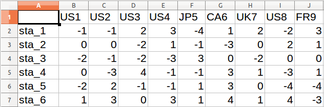
The table shall have the following structure: statements as rows, Q-sorts as columns, and the scores of each Q-sort for each statement in the cells (as in the image).

Export it into *.CSV format, for example: mydata.csv. This format is most versatile and is the format used in this cookbook. Any other format is fine, as long as it can be imported in R.

Note: For the analysis, the data should only contain numbers. Column A in the image above contains the names of rows and requires setting row names (e.g. using row.names(), as explained in step 6A below). Row names are useful to navigate and interpret the results. However, if you want to skip setting row names, then delete any column in the CSV containing them.

Alternatively, if you have introduced your data in PQMethod, find the *.DAT file of your project, e.g. myproject.dat, and use function import.pqmethod() to import your data. If you have collected data online using either FlashQ, HTMLQ or easy-htmlq, find the relevant *.CSV or *.JSON data, and use functions import.HTMLQ() or import.easyhtml() to import your data.

If you do not have one synthetic table as above, but only individual, raw Q sorts, you can use the import.q.sorts() function to build such a matrix with items as rows, and participants as columns. For more information, see the page on data management.

Note: You can also introduce the data directly in R. The way to do it is excluded from this cookbook because it is covered elsewhere in introductory courses for R.

2. Install R

See full details in CRAN - R project. If you wish to use a Graphical User Interface (GUI) for R rather than pure command lines, try R Commander, Deducer, RKWard or RStudio. However, all the code you need to know is below.

Example of the R console. ***

3. Install the package (only once)

Copy the code below and paste it in the R console:

install.packages("qmethod")

4. Load the package (every time you open R)

Copy the code below and paste it in the R console:

library(qmethod)

5. Set your working directory

The working directory is where your files are located, and where your results and plots will be exported.

setwd("your_path")

You should replace your_path with the location of your folder. In Linux and Mac it will be something like setwd("/home/johnbrown/MyQstudy"). In Windows it will be something like setwd("C://MyDocuments/MyQStudy")

If you are using a GUI such as R Studio, you can set the working directory by using the menus. In RStudio go to Session > Set Working Directory > Choose Directory.

6. Import your data into R

There are a number of options, depending on the format of your data.

Below are examples of code, you will need to adapt those examples to your particular file names etc. To import other formats not indicated below (such as SPSS, Excel, or Stata), see Quick R.

A. Import from CSV

See help(read.csv) for help on additional arguments, such as whether the first row of your data is the name of the columns, etc.

mydata <- read.csv("mydata.csv")

# If needed, set the row names. For example, if the first column contains row names, use:
# row.names(mydata) <- mydata[ ,1]
# Then delete the first column, so that the matrix or data frame contains only numbers:
# mydata[ ,1] <- NULL

B. Import from other Q software

From PQMethod:

mydata <- import.pqmethod("myproject.dat")

From both FlashQ and HTMLQ:

# The following imports the Q-sorts only:
mydata <- import.htmlq("myproject.csv")[[1]]

# to see other data related to the P-set, change [[1]] to [[2]]

From easy-htmlq:

# The following imports the Q-sorts only:
mydata <- import.easyhtmlq("myproject.json")[[1]]

# to see other data related to the P-set, change [[1]] to [[2]]

C. Introduce Q-sorts manually

# Create one vector for each Q-sort:
qsort1 <- c(-1,  0, -2,  0, -2, ...)
qsort2 <- c(-1,  0, -1, -3,  2, ...)
...

# Bind all the Q-sorts together:
mydata <- cbind(qsort1, qsort2, ...)

D. Import from Raw Q-Sorts as CSV

You can use the functions import.q.concourse, import.q.sorts, import.q.feedback and build.q.set to import everything from raw *.CSV (and *.TEX) files start your project from scratch, and automatically. For more information, see the page on data management.

Check that the data are correctly imported:

# See the number of statements and of Q-sorts:
dim(mydata)

# See the whole dataset:
mydata

7. Explore the correlations between Q-sorts

You can choose the correlation method from either: Pearson, Kendall or Spearman (Pearson being the default option).

See the help page for the function cor() for more details.

cor(mydata) 

8. Explore the factor loadings

This will help you decide whether to do automatic or manual flagging. For details on how to run the analysis with manual flagging or how to change the loadings, see Advanced analysis.

# Run the analysis
# Create an object called 'results', and put the output 
# of the function 'qmethod()' into this object
# (replace the number of factor 'nfactors' as necessary)
results <- qmethod(mydata, nfactors = 3)

# See the factor loadings
round(results$loa, digits = 2)

# See the flagged Q-sorts: those indicating 'TRUE'
results$flag

Additionally, you can print the loadings and the flags next to each other using the function loa.and.flags:

# Print the table of factor loadings with an indication of flags, 
# as extracted from the object results$flag:
loa.and.flags(results)

Note the qmethod() function uses “PCA” extraction and “varimax” rotation by default, but these attributes can be changed easily (see help(qmethod) for full details; attribute extraction in qmethod package versions >=1.7 only).

# Run the analysis using centroid factor extraction instead of PCA, and without rotation:
results <- qmethod(mydata, nfactors = 3, extraction="centroid", rotation="none")

# Explore using the code above

9. Decide upon the number of factors to extract

See more about the criteria to decide on the number of factors in Watts & Stenner (2012, pp.105-110).

A. Eigenvalues, total explained variability, and number of Q-sorts significantly loading

results$f_char$characteristics
# Column 'eigenvals': eigenvalues
# Column 'expl_var':  percentage of explained variability
# Column 'nload':     number of Q-sorts flagged

B. Screeplot

The following example works for PCA only:

screeplot(prcomp(mydata), main = "Screeplot of unrotated factors", 
          type = "l")

10. Run the final analysis

Once the final number of factors has been decided, run the analysis again.

The method below uses by default Pearson coefficient for the initial correlation, “PCA” extraction and “varimax” rotation; you can change these in the arguments extraction, rotation and cor.method. See help(qmethod) for full details (attribute extraction in qmethod package versions >=1.7 only).

A. Studies with forced distribution

# Create an object called 'results', and put the output 
# of the function 'qmethod' into this object:`
results <- qmethod(mydata, nfactors = 3)

B. Studies with non-forced distribution

# Create a vector with the scores of the expected distribution
distro <- c(-3, -3, -2, -2, -2, -1, -1, -1,  0, ... )

# Create an object called 'results', and put the output 
# of the function 'qmethod' into this object:`
results <- qmethod(mydata, nfactors = 3, 
                   forced = FALSE, 
                   distribution = distro)

11. Explore the results

A. Summary: general characteristics and factor scores

summary(results)

B. Full results

See details of all the objects in the results in Zabala (2014, pp. 167).

results

C. Plot the z-scores for statements

Statements are sorted from highest consensus (bottom) to highest disagreement (top).

plot(results)

D. Reorder the statements from highest to lowest scores for each factor

# Put z-scores and factor scores together
scores <- cbind(round(results$zsc, digits=2), results$zsc_n)
nfactors <- ncol(results$zsc)
col.order <- as.vector(rbind(1:nfactors, (1:nfactors)+nfactors))
scores <- scores[col.order]
scores

# Order the table from highest to lowest z-scores for factor 1
scores[order(scores$zsc_f1, decreasing = T), ]
# (to order according to other factors, replace 'f1' for 'f2' etc.)

E. Explore the table of distinguishing and consensus statements

See a detailed explanation of this table in Zabala (2014, pp. 167-8).

# Full table
results$qdc

# Consensus statements
results$qdc[which(results$qdc$dist.and.cons == "Consensus"), ]

# Statements distinguishing all factors
results$qdc[which(results$qdc$dist.and.cons == "Distinguishes all"), ]

# Statements distinguishing factor 1 (for results of > 2 factors)
results$qdc[which(results$qdc$dist.and.cons == "Distinguishes f1 only"), ]

12. Export the results

A. In R data format

save(results, file = "myresults.Rdata")

# Load them again
load("myresults.Rdata")

B. Individual tables to be imported into a spreadsheet

See all the tables in the results that can be exported in Zabala (2014, pp. 167), or by looking at the structure of your results str(results).

# Table of z-scores:
write.csv(results$zsc,   file = "zscores.csv")

# Table of factor scores:
write.csv(results$zsc_n, file = "factorscores.csv")

# Table of Q-sort factor loadings:
write.csv(results$loa,   file = "loadings.csv")

C. Report of all results (text file)

export.qm(results, file = "myreport.txt", style = "R")

D. Report of results (text file) with the structure of a PQMethod report

This is equivalent to the report in a *.LIS file.

export.qm(results, file = "myreport-pqm.txt", style = "PQMethod")